Building a web app - Part 1 Supporting tagline
I’d like to start off this series of posts by taking a look at the data we’re going to be working with. As a reminder, I’m sharing the code for this series at https://github.com/dkincaid/web-app-explore.
As I mentioned last post the data that we’re going to use comes from the Tycho project at University of Pittsburgh. I’m going to use the Level 2 data. I chose this data for a couple reasons. The first is that it is a little larger dataset (47 diseases over 1888-2013) and offers an API to access the data.
For more information on this data see:
Willem G. van Panhuis, John Grefenstette, Su Yon Jung, Nian Shong Chok, Anne Cross, Heather Eng, Bruce Y Lee, Vladimir Zadorozhny, Shawn Brown, Derek Cummings, Donald S. Burke. Contagious Diseases in the United States from 1888 to the present. NEJM 2013; 369(22): 2152-2158.
Overview
I have already downloaded and processed all the data for all the states into a file named
states_cases.Rda. Let’s load that up and have a look.
options(width = 120, warn = -1)
load("states_cases.Rda")
str(states_cases)
## 'data.frame':	819885 obs. of  6 variables:
##  $ year   : chr  "1942" "1942" "1942" "1942" ...
##  $ week   : chr  "1" "2" "3" "4" ...
##  $ state  : Factor w/ 57 levels "AL","AR","AZ",..: 1 1 1 1 1 1 1 1 1 1 ...
##  $ number : int  0 0 0 0 0 0 0 0 0 0 ...
##  $ event  : Factor w/ 1 level "CASES": 1 1 1 1 1 1 1 1 1 1 ...
##  $ disease: Factor w/ 39 levels "ANTHRAX","BOTULISM",..: 1 1 1 1 1 1 1 1 1 1 ...
summary(states_cases)
##      year               week               state            number        event
##  Length:819885      Length:819885      NY     : 82686   Min.   :    0   CASES:819885
##  Class :character   Class :character   CA     : 22953   1st Qu.:    1
##  Mode  :character   Mode  :character   TX     : 21116   Median :    5
##                                        OH     : 20316   Mean   :   65
##                                        FL     : 20070   3rd Qu.:   28
##                                        MI     : 19188   Max.   :89363
##                                        (Other):633556
##                           disease
##  MEASLES                      :118727
##  WHOOPING COUGH [PERTUSSIS]   : 75424
##  DIPHTHERIA                   : 65007
##  SCARLET FEVER                : 64310
##  SMALLPOX                     : 53461
##  TYPHOID FEVER [ENTERIC FEVER]: 41711
##  (Other)                      :401245
So we have counts of the number of cases reported in each state for each week of the year. What is the range of years?
c(min(states_cases$year), max(states_cases$year))
## [1] "1900" "2013"
Let’s see how the total cases for each disease in the data. Here I’m going to use the new package
from Hadley Wickam, dplyr (which I am loving!).
library(dplyr, quietly = TRUE, warn.conflicts = FALSE)
states_cases %.% group_by(disease) %.% summarise(total = sum(number)) %.% arrange(desc(total))
## Source: local data frame [39 x 2]
##
##                               disease    total
## 1                             MEASLES 22591587
## 2                           INFLUENZA  6741366
## 3                           CHLAMYDIA  5237336
## 4                       SCARLET FEVER  5166016
## 5                           GONORRHEA  4117671
## 6          WHOOPING COUGH [PERTUSSIS]  2813601
## 7              CHICKENPOX [VARICELLA]  1808532
## 8                               MUMPS   914045
## 9                          DIPHTHERIA   910819
## 10          STREPTOCOCCAL SORE THROAT   638494
## 11                            RUBELLA   479160
## 12 TUBERCULOSIS [PHTHISIS PULMONALIS]   300760
## 13                          PNEUMONIA   286079
## 14      TYPHOID FEVER [ENTERIC FEVER]   259413
## 15                           SMALLPOX   242003
## 16                      SALMONELLOSIS   205408
## 17                  RABIES IN ANIMALS   148768
## 18                       LYME DISEASE   128033
## 19                         GIARDIASIS    96853
## 20                        SHIGELLOSIS    68185
## 21                          DYSENTERY    56341
## 22                            MALARIA    37629
## 23       BRUCELLOSIS [UNDULANT FEVER]    35940
## 24                 COCCIDIOIDOMYCOSIS    34481
## 25                  CRYPTOSPORIDIOSIS    30581
## 26       ROCKY MOUNTAIN SPOTTED FEVER    28198
## 27                      LEGIONELLOSIS    20464
## 28                          TULAREMIA    17088
## 29                       TYPHUS FEVER    16220
## 30                         MENINGITIS     4456
## 31                            TETANUS     2639
## 32                       TRICHINIASIS     2027
## 33               TOXIC SHOCK SYNDROME     1957
## 34                        PSITTACOSIS     1345
## 35                            ANTHRAX      204
## 36                            LEPROSY      150
## 37                      POLIOMYELITIS       64
## 38                           BOTULISM       15
## 39                           PELLAGRA        0
and what about the top 10 years?
states_cases %.% group_by(year) %.% summarise(total = sum(number)) %.% arrange(desc(total)) %.% head(10)
## Source: local data frame [10 x 2]
##
##    year   total
## 1  1941 2063853
## 2  1928 1755548
## 3  1938 1738608
## 4  1943 1527009
## 5  1939 1490709
## 6  1929 1381464
## 7  1935 1359174
## 8  1946 1358645
## 9  1944 1344990
## 10 1973 1264263
How about looking at the worst 10 years for each disease (I’ll just show the first 3 diseases here to save some space)
topyear <- function(d) {
    subset(states_cases, disease == d) %.% group_by(year) %.% summarise(total = sum(number)) %.% arrange(desc(total)) %.% head(10)
}

topyears.by.disease <- lapply(levels(states_cases$disease), topyear)
names(topyears.by.disease) <- levels(states_cases$disease)
head(topyears.by.disease, 3)
## $ANTHRAX
## Source: local data frame [4 x 2]
##
##   year total
## 1 1943    90
## 2 1942    67
## 3 1944    45
## 4 1945     2
##
## $BOTULISM
## Source: local data frame [1 x 2]
##
##   year total
## 1 1952    15
##
## $`BRUCELLOSIS [UNDULANT FEVER]`
## Source: local data frame [10 x 2]
##
##    year total
## 1  1947  6436
## 2  1946  5830
## 3  1945  4623
## 4  1948  2631
## 5  1952  2098
## 6  1953  1823
## 7  1954  1812
## 8  1955  1266
## 9  1956  1091
## 10 1957   915
So we can see that for each disease we have very different amounts of data. Let’s see what the min and max year is for each disease
states_cases %.% group_by(disease) %.% summarise(min = min(year), max = max(year), range = as.numeric(max) - as.numeric(min)) %.% arrange(disease)
## Source: local data frame [39 x 4]
##
##                               disease  min  max range
## 1                             ANTHRAX 1942 1945     3
## 2                            BOTULISM 1952 1952     0
## 3        BRUCELLOSIS [UNDULANT FEVER] 1945 1981    36
## 4              CHICKENPOX [VARICELLA] 1972 2013    41
## 5                           CHLAMYDIA 2006 2013     7
## 6                  COCCIDIOIDOMYCOSIS 2006 2013     7
## 7                   CRYPTOSPORIDIOSIS 2006 2013     7
## 8                          DIPHTHERIA 1920 1981    61
## 9                           DYSENTERY 1942 1948     6
## 10                         GIARDIASIS 2006 2013     7
## 11                          GONORRHEA 1972 2013    41
## 12                          INFLUENZA 1919 1951    32
## 13                      LEGIONELLOSIS 1982 2013    31
## 14                            LEPROSY 1942 1945     3
## 15                       LYME DISEASE 2006 2013     7
## 16                            MALARIA 1952 2013    61
## 17                            MEASLES 1909 1982    73
## 18                         MENINGITIS 1917 1959    42
## 19                              MUMPS 1968 2013    45
## 20                           PELLAGRA 1928 1929     1
## 21                          PNEUMONIA 1920 1951    31
## 22                      POLIOMYELITIS 1939 1939     0
## 23                        PSITTACOSIS 1956 1961     5
## 24                  RABIES IN ANIMALS 1948 2013    65
## 25       ROCKY MOUNTAIN SPOTTED FEVER 1942 2011    69
## 26                            RUBELLA 1966 2001    35
## 27                      SALMONELLOSIS 2006 2013     7
## 28                      SCARLET FEVER 1909 1966    57
## 29                        SHIGELLOSIS 2006 2013     7
## 30                           SMALLPOX 1900 1952    52
## 31          STREPTOCOCCAL SORE THROAT 1960 1961     1
## 32                            TETANUS 1962 1972    10
## 33               TOXIC SHOCK SYNDROME 1983 1994    11
## 34                       TRICHINIASIS 1952 1955     3
## 35 TUBERCULOSIS [PHTHISIS PULMONALIS] 1921 2013    92
## 36                          TULAREMIA 1942 1973    31
## 37      TYPHOID FEVER [ENTERIC FEVER] 1909 1983    74
## 38                       TYPHUS FEVER 1942 1947     5
## 39         WHOOPING COUGH [PERTUSSIS] 1909 2013   104
Graphical visualizations
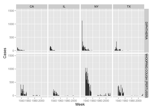
Finally, let’s look at a couple of plots. Here is a look at diphtheria and whooping cough in the states of New York, California, Texas and Illinois.
library(ggplot2, quietly = TRUE)
di <- c("DIPHTHERIA", "WHOOPING COUGH [PERTUSSIS]")

dip_whoop <- subset(states_cases, disease %in% di & state %in% c("NY", "CA", "TX", "IL"))

ggplot(dip_whoop, aes(x = as.Date(paste("1", week, year, sep = "-"), format = "%w-%W-%Y"), y = number)) + geom_bar(stat = "identity", width = 7) + scale_y_continuous("Cases", limits = c(0,
    1500)) + scale_x_date("Week") + facet_grid(disease ~ state)
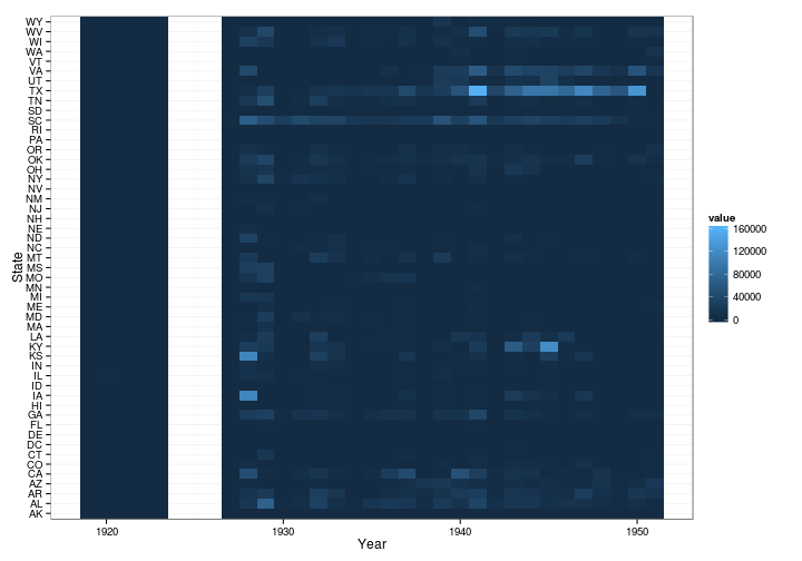
Now I’ll create a matrix for Whooping Cough with states as rows and years as columns and create a heatmap.
library(reshape2, quietly = TRUE, warn.conflicts = FALSE)
library(RColorBrewer, quietly = TRUE, warn.conflicts = FALSE)
influenza.year.by.state <- acast(subset(states_cases, disease == "INFLUENZA"), state ~ year, value.var = "number", fun.aggregate = sum)
influenza.year.by.state[1:10, 1:10]
##    1919 1920 1921 1922 1923 1927  1928  1929 1930  1931
## AL   15    0    0    0    0  416 15705 69455 3281  5925
## AR  213   88    0    0    0  404 12323 20058 2529  3504
## AZ    0    0    0    0    0    1  4347   628  348   462
## CA  182  288    0    0    0  112 44906  5398 1716  5987
## CO    0    0    0    0    0    2  5677   998   11     0
## CT   60   15    0    0    0   49  1068 16748  251  1300
## DC    0  126    0    0    0    0   571  2028   36   219
## DE   14    1    0    0    0    3    43   486   18   275
## FL  114   12    0    0    0   39  1614  3737  104  1496
## GA  204   54    0    0    0  467 23688 29033 3348 12325
m <- melt(influenza.year.by.state)

ggplot(m, aes(x = Var2, y = Var1, fill = value)) + geom_tile() + scale_colour_brewer() + labs(x = "Year", y = "State", color = "Cases") + theme_bw()
Next time
I think that is enough for now. That should give you a decent sense for the data we’ll be working with. Next time I’ll start creating the Shiny application that will let someone do some of this exploration on a web based UI.
blog comments powered by Disqus